Chemotaxis of bacteria is a molecular mechanism by which they sense chemicals and swim through a biased random walk toward preferred concentrations. It has been studied extensively since late 60-s and became a triumph of quantitative system biology, thanks to giants like Julius Adler, Howard C. Berg, Daniel Koshland, to name a few.
Perhaps the most instrumental in this scientific revolution was Howard Berg’s tracking microscope (Berg 1971; PDF), which could follow a freely swimming E.coli cell in 3D in real time. Yes, in 1971. It allowed precise quantification of cell swimming trajectories in spatial and temporal gradients of chemicals, which led to discovery that E.coli performs a biased random walk, with longer runs toward increasing concentrations of attractive chemicals (Berg and Brown, 1972; PDF). This work laid the foundation of quantitative approach to bacterial chemotaxis, which led to multiple breakthroughs on it’s biochemical and physical mechanisms.
Even today in 2017, building a tracking microscope which keeps a rapidly swimming organism in focus is not an easy task. The system had to keep track of rapidy swimming bacterium within a very small depth of field and accurately update servo positions with at least 50 Hz frequency (20 ms intervals). Fast sCMOS cameras, real-time operating system, LabView, FPGA, and C/C++ were unknown words in the late 1960-s. Computers were using punch cards and magnetic tapes.
In a stunning tour de force Howard Berg created a tracking microscope using only optic fibers, photomultipliers, off-the-shelf analog electronic components, and electomagnetic coils on top of a Nikon upright microscope, at a cost about $5K (equivalent of ~30K in 2017). Machining and electronics he did himself. The tracking data were stored using an oscilloscope or magnetic tapes.

“The scene through the binocular is extraordinary. The bacterium being tracked seems to be stuck to the center of the field, turning this way and that trying to free itself, while the other bacteria drift in and out of focus, then to and from, in apparent synchrony. If the bacterium being tracked is long, it seems to be stuck at one end and then at the other; the microscope will track on any part.” (Berg 1971)
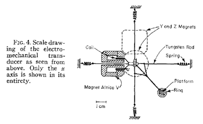
Fast and precise piezo stages? None in 1971. Use coils and cylindrical magnets, springs and rods. Ah, don't forget to make the rods from tungsten - they should be non-magnetic and stiff.
Berg's tracking microscope is an inspiration and example of scientific instrumentation mastery - bold ideas and finesse of implementation, applied for making groundbreaking discoveries in biology. Prof. Howard C Berg devoted his long career to the amazing world of bacteria, molecular mechanisms of chemotaxis and flaggelar motors, and his book Random Walks in Biology is an all-time classic, where physics marries biology.
Perhaps the most instrumental in this scientific revolution was Howard Berg’s tracking microscope (Berg 1971; PDF), which could follow a freely swimming E.coli cell in 3D in real time. Yes, in 1971. It allowed precise quantification of cell swimming trajectories in spatial and temporal gradients of chemicals, which led to discovery that E.coli performs a biased random walk, with longer runs toward increasing concentrations of attractive chemicals (Berg and Brown, 1972; PDF). This work laid the foundation of quantitative approach to bacterial chemotaxis, which led to multiple breakthroughs on it’s biochemical and physical mechanisms.
Even today in 2017, building a tracking microscope which keeps a rapidly swimming organism in focus is not an easy task. The system had to keep track of rapidy swimming bacterium within a very small depth of field and accurately update servo positions with at least 50 Hz frequency (20 ms intervals). Fast sCMOS cameras, real-time operating system, LabView, FPGA, and C/C++ were unknown words in the late 1960-s. Computers were using punch cards and magnetic tapes.

In a stunning tour de force Howard Berg created a tracking microscope using only optic fibers, photomultipliers, off-the-shelf analog electronic components, and electomagnetic coils on top of a Nikon upright microscope, at a cost about $5K (equivalent of ~30K in 2017). Machining and electronics he did himself. The tracking data were stored using an oscilloscope or magnetic tapes.

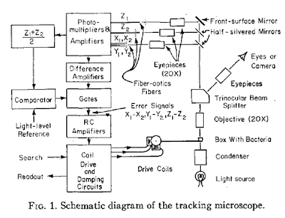
The principle of tracking H.Berg proposed was simple and elegant. A phase-contrast image of a bacterium is relayed onto 3 pairs of photomultipliers (PMTs), x1, x2, y1, y2, z1, z2. Displacement of the bacterium in +x direction excites the x1 PMT, so the difference between x1-x2 PMTs is high - it is then amplified and fed into the electromagnetic drive coil which moves the chamber with bacteria. This feedback loop returns the bacteria back to the center of visual field. In z direction, when bacteria swims up it’s image becomes more focused on PMT z1, the difference of signals z1-z2 is amplified and fed into the drive coil for z axis. If bacteria swims beyond the range of drive coils, the microscope automatically returns to the center position and waits for another bacteria to swim by to start a new tracking.
“The scene through the binocular is extraordinary. The bacterium being tracked seems to be stuck to the center of the field, turning this way and that trying to free itself, while the other bacteria drift in and out of focus, then to and from, in apparent synchrony. If the bacterium being tracked is long, it seems to be stuck at one end and then at the other; the microscope will track on any part.” (Berg 1971)
How was this all possible?
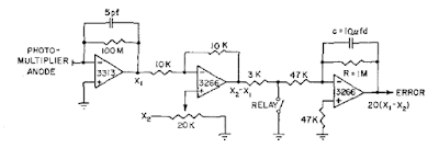
The exact details on how to tune all the analog control loops, select the right materials and components are hard to grasp by us, the digital generation. Real-time LabView with FPGA? Use op-amps, resistors and capacitors instead.
Fast and precise piezo stages? None in 1971. Use coils and cylindrical magnets, springs and rods. Ah, don't forget to make the rods from tungsten - they should be non-magnetic and stiff.

Berg's tracking microscope is an inspiration and example of scientific instrumentation mastery - bold ideas and finesse of implementation, applied for making groundbreaking discoveries in biology. Prof. Howard C Berg devoted his long career to the amazing world of bacteria, molecular mechanisms of chemotaxis and flaggelar motors, and his book Random Walks in Biology is an all-time classic, where physics marries biology.
 |
| A projection of the track of a wildtype E. coli obtained with a microscope which automatically follows its motion in three dimensions (from H.C.Berg's website). |
Comments
Post a Comment